Appearance
Back Propagation
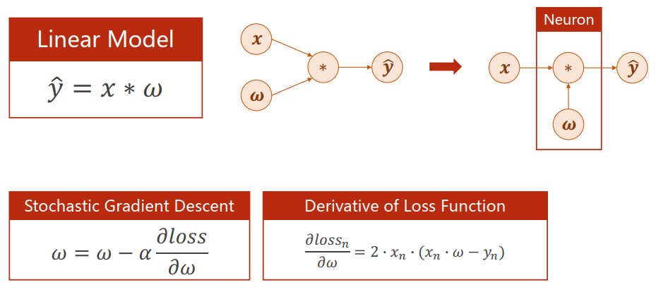
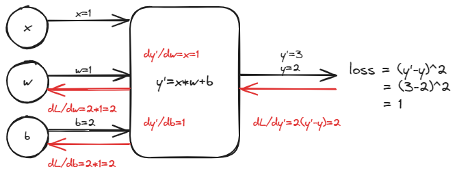
Compute gradient in simple network
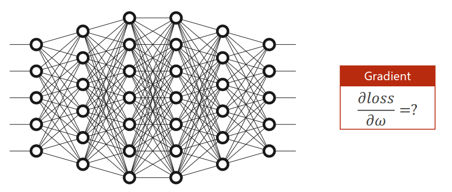
What about the complicated network?
在复杂网络中,把每一个权重梯度的解析式写出来是不可能的,要使用新的方法进行处理。
反向传播(BP, back propagation)是一种用来训练人工神经网络的常见方法,它是一种与最优化方法(如梯度下降法)结合使用的。在训练过程中,神经网络根据输入数据和目标输出计算损失函数,然后通过反向传播算法计算损失函数对每一个参数的梯度。
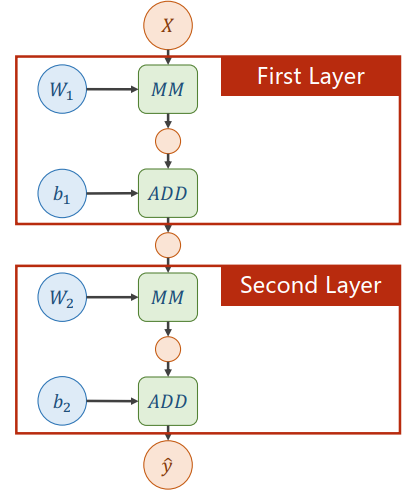
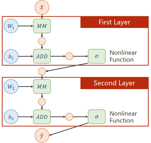
Computational Graph
A two layer neural network:
Note
矩阵梯度计算公式查看->matrixcookbook.pdf (uwaterloo.ca)
What problem about this two layer neural network?
尝试进行如下计算:
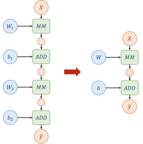
发现任何多层的网络都可以经过线性变化简化为一层,但是这使得增加的权重失去了意义。
所以需要对每层的输出增加一个非线性的变化函数。
The composition of functions and Chain Rule
链式求导法则(chain rule):
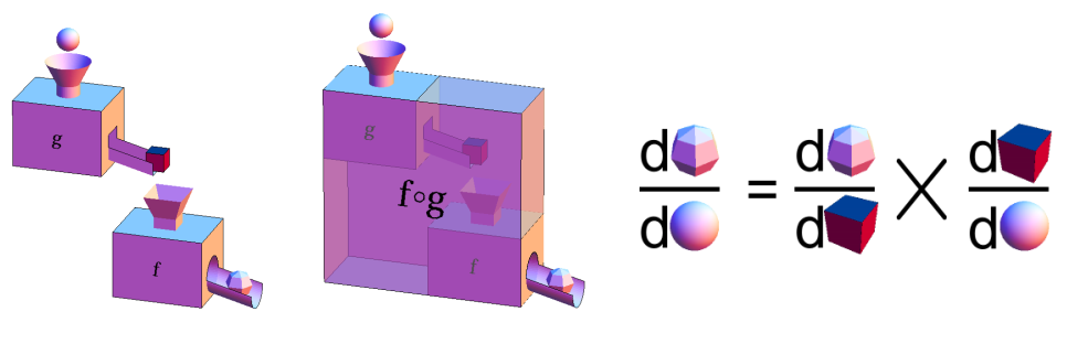
在神经网络中,forward计算损失,再用链式法则backward计算梯度。
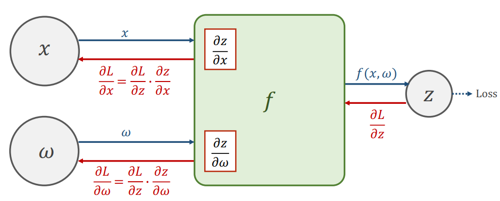
Note
为什么要计算x的梯度?x作为数据输入无需计算梯度,但是x作为中间结果是上一层的输出时,是需要知道它的梯度的。
Example
举例1:,假设,猜测
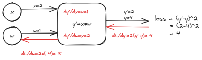
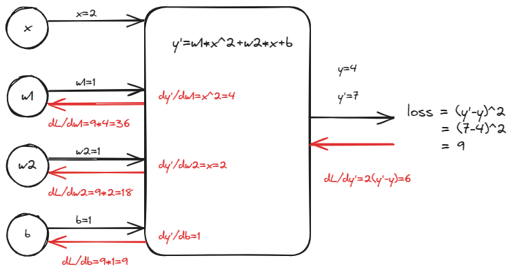
举例2:,假设,猜测
Tensor in PyTorch
In PyTorch, Tensor is the important component in constructing dynamic computational graph.
It contains data and grad, which storage the value of node and gradient w.r.t loss respectively.
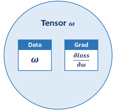
Tensor(即张量)实际上是一种数据类型,有两个重要的成员data和grad,data保存权重本身,grad保存损失函数对权重的导数。
Implementation of linear model with PyTorch
代码:
import torch

x_data = [1.0, 2.0, 3.0]
y_data = [2.0, 4.0, 6.0]

w = torch.Tensor([1.0])    # 权重初始化为1.0
w.requires_grad = True


def forward(x): return x * w


def loss(x, y):
    y_pred = forward(x)
    return (y_pred - y) ** 2


print("predict (before training)", 4, forward(4).item())

for epoch in range(100):
    for x, y in zip(x_data, y_data):
        l = loss(x, y)                         # forward,构建计算图计算loss
        l.backward()                           # backward
        print('\tgrad:', x, y, w.grad.item())
        w.data = w.data - 0.01 * w.grad.data   # 梯度下降
        w.grad.data.zero_()                    # 清零
    print("progress:", epoch, l.item())

print("predict (after training)", 4, forward(4).item())
Exercise
Quadratic Model:
Loss Function:
反向传播过程:
代码实现:
import torch

x_data = [1.0, 2.0, 3.0]
y_data = [2.0, 4.0, 6.0]

w1 = torch.Tensor([1.0])
w1.requires_grad = True
w2 = torch.Tensor([1.0])
w2.requires_grad = True
b = torch.Tensor([1.0])
b.requires_grad = True


def forward(x):
    return w1 * (x ** 2) + w2 * x + b


def loss(x, y):
    y_pred = forward(x)
    return (y_pred - y) ** 2


print("predict (before training)", 4, forward(4).item())

for epoch in range(100):
    for x, y in zip(x_data, y_data):
        l = loss(x, y)
        l.backward()
        print('\tgrad:', x, y, w1.grad.item(), w2.grad.item(), b.grad.item())
        w1.data = w1.data - 0.01 * w1.grad.data
        w2.data = w2.data - 0.01 * w2.grad.data
        b.data = b.data - 0.01 * b.grad.data
        w1.grad.data.zero_()
        w2.grad.data.zero_()
        b.grad.data.zero_()
    print("progress:", epoch, l.item())

print("predict (after training)", 4, forward(4).item())