逻辑斯蒂回归（Logistic Regression）解决的是分类问题。

Regression vs Classification

回归问题中$y\in R$，而分类问题中类别之间无法比较大小。

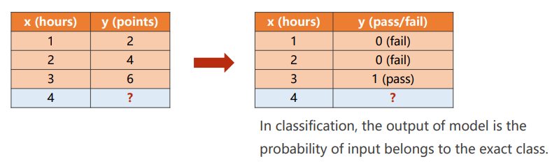
通过计算属于每个分类的概率来处理分类问题，预测属于概率最高的那个分类。

继续之前的例子，改造为二分类问题。

Sigmoid functions

How to map: R->[0,1]?

Logistic Function:

$$\sigma(x)=\frac{1}{1+e^{-x}}$$

该函数的图像如下图所示：

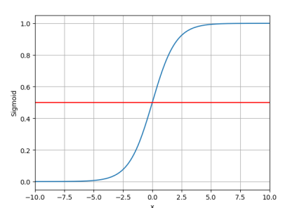
将$\hat y=\omega x+b$代入Logistic Function，就可以将实数映射到[0,1]范围内。

Tips

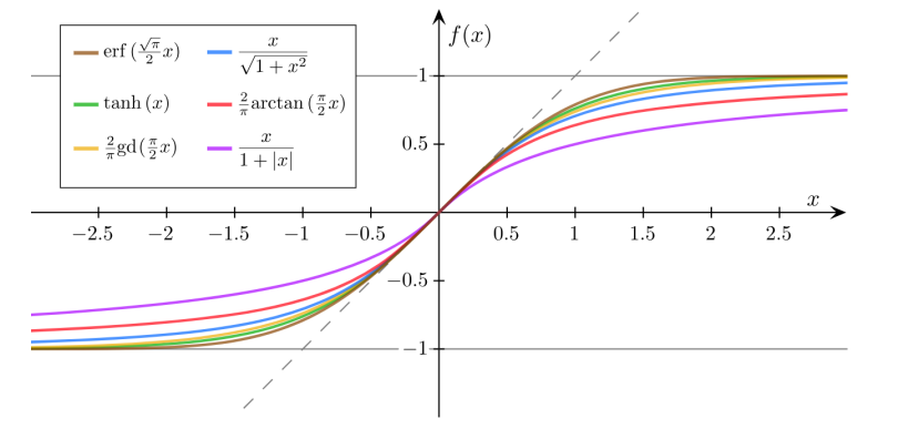
经常将Logistic Function称为Sigmoid Function，但是实际上Sigmoid Function不只有Logistic Function。

以下函数也可以作为Sigmoid Function：

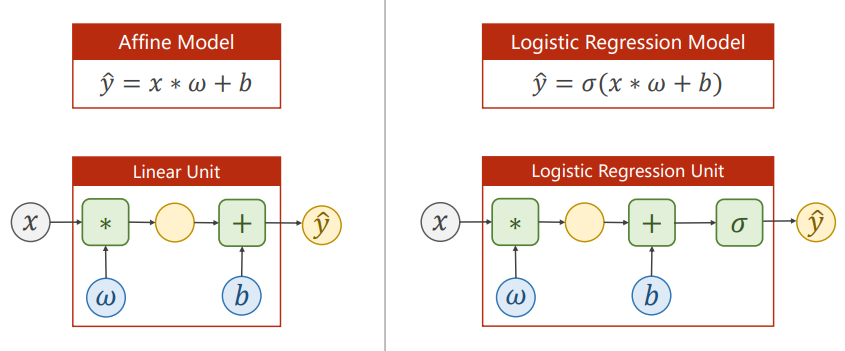
Logistic Regression Model

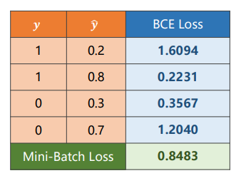
Loss Function for Binary Classification

$$loss=-(y\log\hat y+(1-y)\log(1-\hat y))$$

• 当实际类别为1时（y=1），$loss=-\log\hat y$，$\hat y$是预测的类别为1的概率
• 当实际类别为0时（y=0），$loss=-\log(1-\hat y)$，$1-\hat y$是预测的类别为0的概率
• 预测正确的概率越大损失越小

Note

交叉熵（cross-entropy）

Mini-Batch Loss Function for Binary Classification

$$loss=-\frac{1}{N}\sum_{n=1}^Ny_n\log\hat y_n+(1-y_n)\log(1-\hat y_n)$$

Implementation of Logistic Regression

import torch  
import numpy as np  
import matplotlib.pyplot as plt  
  
x_data = torch.Tensor([[1.0], [2.0], [3.0]])  
y_data = torch.Tensor([[0], [0], [1]])  
  
  
class LinearModel(torch.nn.Module):  
    def __init__(self):  
        super().__init__()  
        self.linear = torch.nn.Linear(1, 1)  
  
    def forward(self, x):  
        y_pred = torch.sigmoid(self.linear(x))  
        return y_pred  
  
  
model = LinearModel()  
criterion = torch.nn.BCELoss(reduction='sum')  
optimizer = torch.optim.SGD(model.parameters(), lr=0.01)  
  
for epoch in range(1000):  
    y_pred = model(x_data)  # Forward: Predict  
    loss = criterion(y_pred, y_data)  # Forward: Loss  
    print(epoch, loss.item())  
    optimizer.zero_grad()  # before backward: set the grad to ZERO  
    loss.backward()  # Backward: Autograd  
    optimizer.step()  # Update  
  
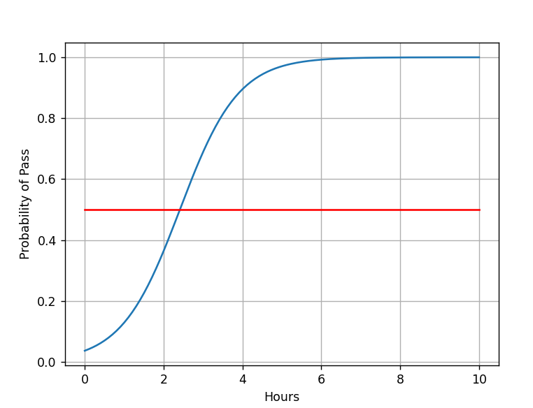
x = np.linspace(0, 10, 200)  
x_t = torch.Tensor(x).view((200, 1))  
y_t = model(x_t)  
y = y_t.data.numpy()  
plt.plot(x, y)  
plt.plot([0, 10], [0.5, 0.5], c='r')  
plt.xlabel('Hours')  
plt.ylabel('Probability of Pass')  
plt.grid()  
plt.show()